01 – Genomic Prediction for Coronary Artery Disease

A - Setup

In this tutorial, we will be using EIR-auto-GP, to train deep learning models for predicting coronary artery disease (CAD) risk based on genotype data and a mix of categorical and continuous tabular inputs (i.e., clinical data).

We will be working with data from the PennCATH study, (here the data obtained gotten from this excellent GWAS tutorial), which investigates genetic risk factors for coronary artery disease. To start, please download the processed PennCATH data (or process your own .bed, .bim, .fam files using EIR-auto-GP). The same approach can be applied to other cohorts and diseases, such as the UK Biobank for other complex trait predictions.

First, let’s set up our folders:

$ mkdir -p eir_auto_gp_tutorials/01_basic_tutorial/data
$ mkdir -p eir_auto_gp_tutorials/tutorial_runs/01_basic_tutorial

Now, the downloaded data should have the following structure:

eir_auto_gp_tutorials/01_basic_tutorial/data
├── penncath
│   ├── penncath.bed
│   ├── penncath.bim
│   ├── penncath.csv
│   └── penncath.fam
└── penncath.zip

Examining the data, we can see that we are working with 861473 SNPs (.bim file) and 1401 individuals (.fam file).

Looking at the corresponding penncath.csv file, we can see the labels for each individual.

"ID","CAD","sex","age","tg","hdl","ldl"
"10002",1,1,60,NA,NA,NA
"10004",1,2,50,55,23,75
"10005",1,1,55,105,37,69
"10007",1,1,52,314,54,108
"10008",1,1,58,161,40,94
"10009",1,1,59,171,46,92
"10010",1,1,54,147,69,109
"10011",1,2,66,124,47,84
"10012",1,1,58,60,114,67

Important

The label file ID column must be called “ID” (uppercase).

So, here we can see the CAD status we want to predict (with 1 being CAD positive), but we also have some more information about the individuals. Namely, we have sex, age, tg (triglycerides), hdl (high density lipoprotein) and ldl (low density lipoprotein).

Before diving into the model training, we’ll first have a quick look at the eir_auto_gp command line interface.

usage: eirautogp [-h] --genotype_data_path GENOTYPE_DATA_PATH
                 [--genotype_processing_chunk_size GENOTYPE_PROCESSING_CHUNK_SIZE]
                 --label_file_path LABEL_FILE_PATH [--only_data]
                 [--global_output_folder GLOBAL_OUTPUT_FOLDER]
                 [--data_output_folder DATA_OUTPUT_FOLDER]
                 [--feature_selection_output_folder FEATURE_SELECTION_OUTPUT_FOLDER]
                 [--modelling_output_folder MODELLING_OUTPUT_FOLDER]
                 [--analysis_output_folder ANALYSIS_OUTPUT_FOLDER]
                 [--output_name OUTPUT_NAME]
                 [--pre_split_folder PRE_SPLIT_FOLDER]
                 [--freeze_validation_set] [--no-freeze_validation_set]
                 [--feature_selection {dl,gwas,gwas->dl,dl+gwas,gwas+bo,None,None}]
                 [--n_dl_feature_selection_setup_folds N_DL_FEATURE_SELECTION_SETUP_FOLDS]
                 [--gwas_p_value_threshold GWAS_P_VALUE_THRESHOLD]
                 [--folds FOLDS] [--input_cat_columns [INPUT_CAT_COLUMNS ...]]
                 [--input_con_columns [INPUT_CON_COLUMNS ...]]
                 [--output_cat_columns [OUTPUT_CAT_COLUMNS ...]]
                 [--output_con_columns [OUTPUT_CON_COLUMNS ...]] [--do_test]

options:
  -h, --help            show this help message and exit
  --genotype_data_path GENOTYPE_DATA_PATH
                        Root path to raw genotype data to be processed
                        (e.g., containing my_data.bed, my_data.fam, my_data.bim).
                        For this example, this parameter should be
                        '/path/to/raw/genotype/data/'.
                        Note that the file names are not included in this path,
                        only the root folder. The file names are inferred, and
                        *only one* set of files is expected.
  --genotype_processing_chunk_size GENOTYPE_PROCESSING_CHUNK_SIZE
                        Chunk size for processing genotype data. Increasingthis value will increase the memory usage, but willlikely speed up the processing.
  --label_file_path LABEL_FILE_PATH
                        File path to label file with tabular inputs and labels to predict.
  --only_data           If this flag is set, only the data processing step will be run.
  --global_output_folder GLOBAL_OUTPUT_FOLDER
                        Common root folder to save data, feature selection and modelling results in.
  --data_output_folder DATA_OUTPUT_FOLDER
                        Folder to save the processed data in and also to read the data fromif it already exists.
  --feature_selection_output_folder FEATURE_SELECTION_OUTPUT_FOLDER
                        Folder to save feature selection results in.
  --modelling_output_folder MODELLING_OUTPUT_FOLDER
                        Folder to save modelling results in.
  --analysis_output_folder ANALYSIS_OUTPUT_FOLDER
                        Folder to save analysis results in.
  --output_name OUTPUT_NAME
                        Name used for dataset.
  --pre_split_folder PRE_SPLIT_FOLDER
                        If there is a pre-split folder, this will be used to
                        split the data into train/val and test sets. If not,
                        the data will be split randomly.
                        The folder should contain the following files:
                          - train_ids.txt: List of sample IDs to use for training.
                          - test_ids.txt: List of sample IDs to use for testing.
                          - (Optional): valid_ids.txt: List of sample IDs to use for validation.
                        If this option is not specified, the data will be split randomly
                        into 90/10 (train+val)/test sets.
  --freeze_validation_set
                        If this flag is set, the validation set will be frozen
                        and not changed between DL training folds.
                        This only has an effect if the validation set is not specified
                        in as a valid_ids.txt in file the pre_split_folder.
                        If this flag is not set, the validation set will be randomly
                        selected from the training set each time in each DL training run fold.
                        This also has an effect when GWAS is used in feature selection.
                        If the validation set is not specified manually or this flag is set,
                        the GWAS will be performed on the training *and* validation set.
                        This might potentially inflate the results on the validation set,
                        particularly if the dataset is small. To turn off this behavior,
                        you can use the --no-freeze_validation_set flag.
  --no-freeze_validation_set
  --feature_selection {dl,gwas,gwas->dl,dl+gwas,gwas+bo,None,None}
                        What kind of feature selection strategy to use for SNP selection:
                          - If None, no feature selection is performed.
                          - If 'dl', feature selection is performed using DL feature importance,
                            and the top SNPs are selected iteratively using Bayesian optimization.
                          - If 'gwas', feature selection is performed using GWAS p-values,
                            as specified by the --gwas_p_value_threshold parameter.
                          - If 'gwas->dl', feature selection is first performed using GWAS p-values,
                            and then the top SNPs are selected iteratively using the DL importance method,
                            but only on the SNPs under the GWAS threshold.
                          - If 'gwas+bo', feature selection is performed using a combination of
                            GWAS p-values and Bayesian optimization. The upper bound of the fraction
                            of SNPs to include is determined by the fraction corresponding to a
                            computed one based on the gwas_p_value_threshold.
  --n_dl_feature_selection_setup_folds N_DL_FEATURE_SELECTION_SETUP_FOLDS
                        How many folds to run DL attribution calculation on genotype data
                        before using results from attributions for feature selection.
                        Applicable only if using 'dl' or 'gwas->dl' feature_selection options.
  --gwas_p_value_threshold GWAS_P_VALUE_THRESHOLD
                        GWAS p-value threshold for filtering if using 'gwas', 'gwas+bo' or 'gwas->dl'
                        feature_selection options.
  --folds FOLDS         Training runs / folds to run, can be a single fold (e.g. 0),
                        a range of folds (e.g. 0-5), or a comma-separated list of 
                        folds (e.g. 0,1,2,3,4,5).
  --input_cat_columns [INPUT_CAT_COLUMNS ...]
                        List of categorical columns to use as input.
  --input_con_columns [INPUT_CON_COLUMNS ...]
                        List of continuous columns to use as input.
  --output_cat_columns [OUTPUT_CAT_COLUMNS ...]
                        List of categorical columns to use as output.
  --output_con_columns [OUTPUT_CON_COLUMNS ...]
                        List of continuous columns to use as output.
  --do_test             Whether to run test set prediction.

That’s a whole lot of text, but don’t worry - we’re not going to read the entire encyclopedia before we start training a couple of models.

B - Training

Now that we have set up our data, and had a quick look at the eir_auto_gp command line interface, we can start training. So just to review, we are going to train a model to predict CAD risk, using genotype and clinical data as inputs to our models.

First, let’s look at the command we will use to train our model:

eirautogp \
--genotype_data_path eir_auto_gp_tutorials/01_basic_tutorial/data/penncath \
--label_file_path eir_auto_gp_tutorials/01_basic_tutorial/data/penncath/penncath.csv \
--global_output_folder eir_auto_gp_tutorials/tutorial_runs/01_basic_tutorial_1 \
--output_cat_columns CAD \
--input_con_columns tg hdl ldl age \
--input_cat_columns sex \
--folds 5 \
--feature_selection gwas->dl \
--n_dl_feature_selection_setup_folds 2 \
--do_test

Now, the first options are pretty self-explanatory – they mainly have to do with the input data and the output directory. Let’s take a quick look at some of the more esoteric options and the reasoning behind them:

1. --folds 0-2: This option specifies the folds to run during cross-validation. The train/validation split is randomly performed for each fold. In this tutorial, we’re running 3 folds (0, 1, and 2) for training and validation. Increasing the number of folds might help us get a more stable estimate of the model’s performance, but it will also increase the runtime.

2. --feature_selection gwas->dl: This option specifies the feature selection strategy to use for SNP selection. In this case, we’re using a two-step approach (gwas->dl) that first performs feature selection using GWAS p-values and then refines the selection using a deep learning (DL) importance method. You might have noticed above that we had 861473 SNPs in our dataset, but only 1401 individuals, this means that we might have relatively big \(p \gg n\), problem. Therefore, filtering the SNPs down first with a GWAS p-value threshold (--gwas_p_value_threshold 1e-4) can help reduce overfitting and greatly improve runtime.

3. --n_dl_feature_selection_folds 1: This option sets the number of folds to run DL feature importance calculation on genotype data before using the results for feature selection in subsequent models. In this case, the DL feature importance calculation is run on the first fold after the GWAS feature selection step. If using --feature_selection dl, the DL feature importance calculation is performed on the full set of SNPs.

4. --do_test: This option, when set, instructs the program to run the test set prediction. Generally we would set this option after everything is finalized and we want to get a final estimate of the model’s performance. In this tutorial, we’ll go ahead and just set it from the beginning.

Now, after this relatively dry explanation of the options (apologies), let’s go ahead and run the training. Running the command above took around 8 minutes on my laptop using a CPU. But then again the GWAS filtered the SNPs down to a manageable number.

Note

Some of the settings above (e.g. n_dl_feature_selection_folds and gwas_p_value_threshold) can be tinkered with, but remember to then turn off the --do_test option, as the test set is only used for final model evaluation.

Note

Here we are using the gwas->dl feature selection strategy, but it might well be that using e.g. a purely GWAS based one, such as the gwas+bo is faster and/or more accurate.

Now running this will produce a pretty crazy amount of output to the terminal, but don’t worry, we’ll go through it all. Assuming that everything went well, we should have a new folder in our eir_auto_gp_tutorials directory called tutorial_runs/01_basic_tutorial:

eir_auto_gp_tutorials/tutorial_runs/01_basic_tutorial_1/
├── analysis
│   ├── CAD_feature_selection.pdf
│   ├── CAD_test_predictions.csv
│   ├── CAD_test_results.csv
│   └── CAD_validation_results.csv
├── data
│   ├── genotype
│   ├── ids
│   └── tabular
├── feature_selection
│   ├── dl_importance
│   ├── gwas_label_file.csv
│   ├── gwas_output
│   └── one_hot_mappings.json
└── modelling
    ├── fold_0
    ├── fold_1
    ├── fold_2
    ├── fold_3
    └── fold_4

We will go through these in the order of data -> modelling -> feature_selection -> analysis.

C - Data Output

The data processing pipeline. Starting with a Plink binary fileset and a tabular label file, the data is split into a train and test set, either randomly or according to a pre-specified split. The data is then processed and organized on the disk, ready to be read by the EIR framework for model training. Prior to the full training pipeline, one can pre-filter the SNPs using a GWAS p-value threshold, with the eirautogwas command line interface.

The data folder contains the parsed genotype and tabular data, split into train and test sets. There is not much more to say about this folder, besides perhaps that you can have a look at the ids folder to see how the IDs have been split into train and test sets.

Note

You can configure the exact train and test split by using the --pre-split-folder option. This option takes a folder containing train_ids.txt and test_ids.txt files, where each file contains a list of IDs to be used for training and testing respectively (one ID per line). The default is a 90/10 train/test set split.

Warning

The default approach is to drop samples that have NA values in any of the columns (missing genotype data is supported). If you want to keep samples with missing tabular data, please impute them first (with values based on the training set) and then use the --pre-split-folder option.

Note

When running on large datasets, it might take a while for the data to be processed. However, the data only has to be processed once, and then subsequent runs can reuse the processed data. The data processing speed might be optimized in the future.

D - Modelling Output

The modelling and feature selection part of the pipeline. The training and validation data are used to train and evaluate the DL models. If GWAS is also used for feature selection (using the --feature_selection gwas->dl option), the GWAS p-values are used to filter the SNPs before the any DL models are trained. A set of \(F\) (controlled by the --n_dl_feature_selection_folds option) DL models are trained on the full set of SNPs (where “full” refers to either the full SNP set or the SNP set after GWAS filtering if that option was specified). The \(F\) models are then used to calculate the importance of each SNP using the DL feature importance / attribution method in EIR. If DL is used for feature selection (using the dl or gwas->dl value for --feature_selection option), the SNPs are iteratively pruned using Bayesian optimization w.r.t validation set performance.

This folder contains the EIR runs for each fold. See the EIR documentation and this example tutorial for more information about the output and how it is generated. Feel free to poke around in these folders to see what’s going on, for example you can see train/validation learning curves, confusion matrices, what the DL neural network architecture looks like, the configurations used for training, and the model’s predictions on the test set. Again, please refer to the EIR documentation for more information.

E - Feature Selection Output

First, let’s take a closer look at what the feature_selection folder contains:

eir_auto_gp_tutorials/tutorial_runs/01_basic_tutorial_1/feature_selection
├── dl_importance
│   ├── dl_attributions.csv
│   ├── manhattan
│   │   └── Aggregated CAD_manhattan.png
│   └── snp_subsets
│       ├── dl_snps_0.txt
│       ├── dl_snps_1.txt
│       ├── dl_snps_2.txt
│       ├── dl_snps_3.txt
│       ├── dl_snps_4.txt
│       ├── dl_snps_fraction_0.txt
│       ├── dl_snps_fraction_1.txt
│       ├── dl_snps_fraction_2.txt
│       ├── dl_snps_fraction_3.txt
│       └── dl_snps_fraction_4.txt
├── gwas_label_file.csv
├── gwas_output
│   ├── gwas.CAD.glm.logistic.hybrid
│   ├── gwas.log
│   ├── plots
│   │   ├── gwas.CAD.glm.logistic.hybrid_manhattan.png
│   │   └── gwas.CAD.glm.logistic.hybrid_qq.png
│   └── snps_to_keep.txt
└── one_hot_mappings.json

Now, we included a GWAS step in our feature selection, so we have a gwas_output folder containing the GWAS results as well as a couple of plots, namely a manhattan plot and a QQ plot.

Note

The significance threshold in the manhattan plot reflects what is set by the --gwas_p_value_threshold option.

Now, since we used a hybrid feature selection strategy (gwas->dl), we also have a dl_importance folder containing the DL feature importance results. One of these files is a manhattan like plot for the DL feature importance / attributions:

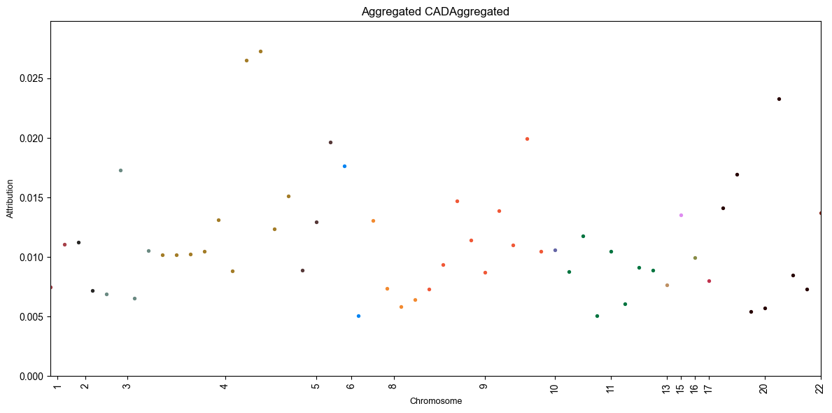
This plot is definitely quite sparse, especially compared to the GWAS manhattan plot above! This is because we only trained the DL models on the SNPs that passed the GWAS p-value threshold from before.

Note

The y-axis here represents the average attribution / feature importance (more specifically, the effect of the SNP on the model’s prediction) across all folds. You can get more information about the specific SNPs and their attributions in the dl_attributions.csv file.

F - Analysis Output

The analysis and test set prediction part of the pipeline. The framework gathers the validation performance results compiles them into a single .csv and as well as an overview figure of the DL feature importance results if applicable. If the --do_test option is specified, the trained DL models from each fold are used to make predictions on the test set, which are reported in the analysis folder as well as an ensemble prediction.

Finally, let’s take a look at the analysis folder:

eir_auto_gp_tutorials/tutorial_runs/01_basic_tutorial_1/analysis
├── CAD_feature_selection.pdf
├── CAD_test_predictions.csv
├── CAD_test_results.csv
└── CAD_validation_results.csv

We will first take a look at the validation performance results:

Validation performance

Fold	Best Avg Perf	ITER	ACC	AP	LOSS	MCC	ROC-AUC	% SNPs
Fold 0	0.7212	700.0	0.8087	0.8238	0.5087	0.564	0.7757	1.0
Fold 1	0.7456	500.0	0.7913	0.8632	0.5354	0.5666	0.807	1.0
Fold 2	0.7339	1550.0	0.7913	0.8634	0.5278	0.54	0.7983	0.6744
Fold 3	0.7408	1600.0	0.8	0.8669	0.4919	0.5486	0.807	0.3242
Fold 4	0.7069	250.0	0.7739	0.8588	0.5353	0.4871	0.7747	0.2857

Note

The best average performance is according to the defaults in EIR, which is average of MCC, ROC-AUC and average precision (AP) for categorical targets and 1.0-LOSS, PCC, R2 for continuous targets.

The DL feature selection method uses Bayesian optimization to select the fraction of SNPs to use, we can see the best average validation performance as a function of the fraction of SNPs used:

Now, the results do not change much between trials, perhaps because we have already filtered the SNPs using GWAS.

In any case, now let’s finally take a look at the test set performance:

Test set performance

Fold	MCC	ACC	ROC-AUC	AP
Ensemble	0.3868	0.7287	0.7996	0.902
Fold 0	0.2718	0.6977	0.7688	0.8934
Fold 1	0.3313	0.6744	0.7669	0.8886
Fold 2	0.4015	0.7209	0.7846	0.874
Fold 3	0.4002	0.7364	0.7766	0.8892
Fold 4	0.2913	0.6822	0.7312	0.8664

So here we can see that the validation performance seems to have been biased, which makes sense considering it was quite small, and we were seeing some fluctuations between folds. We can see the test set predictions for the individual folds, as well as an ensemble of all the folds.

If you read this far, thank you for your patience! Hopefully you found this tutorial useful!

Appendix – Validation Set Strategy

The default validation set strategy, 10% of the full training data (with a lower threshold of 16-64, depending on the dataset size, and an upper threshold of 20,000) is allocated for validation purposes, while the remaining 90% is utilized for training. This split is consistently maintained across all folds, ensuring that the validation set size remains constant. This approach not only contributes to the model training process but also plays a role in the execution of GWAS. Specifically, GWAS is applied exclusively to the training set.

Alternatively, you can opt for an approach that involves randomly splitting the full training data into training and validation sets during each fold. This method, which can be activated by setting the --no-freeze-validation-set option, allows for independent data splits in each fold. Consequently, the validation set differs for every fold, providing a more varied evaluation of the model’s performance.

eirautogp \
--genotype_data_path eir_auto_gp_tutorials/01_basic_tutorial/data/penncath \
--label_file_path eir_auto_gp_tutorials/01_basic_tutorial/data/penncath/penncath.csv \
--global_output_folder eir_auto_gp_tutorials/tutorial_runs/01_basic_tutorial_2/ \
--output_cat_columns CAD \
--input_con_columns tg hdl ldl age \
--input_cat_columns sex \
--folds 5 \
--feature_selection gwas->dl \
--n_dl_feature_selection_setup_folds 2 \
--do_test \
--no-freeze_validation_set

However, as we no longer have a set training set, the GWAS is applied to the full training data, which includes the validation set. Although this grants the GWAS access to more data, it may result in overfitting concerning the validation set (i.e., the GWAS feature selection has had access to the validation data). While we still have the final test set to get an unbiased estimate of the model’s performance, the validation results may be less reliable. This becomes less of a problem when using larger datasets, but important to keep in mind when using smaller datasets.

We can see the results of this approach below:

Validation performance

Fold	Best Avg Perf	ITER	ACC	AP	LOSS	MCC	ROC-AUC	% SNPs
Fold 0	0.8867	950.0	0.8974	0.9689	0.3348	0.7593	0.9321	1.0
Fold 1	0.7228	350.0	0.7949	0.8283	0.5334	0.5677	0.7722	1.0
Fold 2	0.9469	1000.0	0.9487	0.9796	0.2968	0.8944	0.9667	0.8901
Fold 3	0.8372	250.0	0.8718	0.9514	0.398	0.6933	0.8669	0.2581
Fold 4	0.9364	1300.0	0.9487	0.9811	0.3656	0.8864	0.9416	0.5649

Test set performance

Fold	MCC	ACC	ROC-AUC	AP
Ensemble	0.3737	0.7209	0.829	0.916
Fold 0	0.3775	0.7054	0.7991	0.9038
Fold 1	0.3698	0.7364	0.8154	0.9086
Fold 2	0.3868	0.7287	0.8193	0.9131
Fold 3	0.3775	0.7054	0.7503	0.8766
Fold 4	0.4434	0.7287	0.765	0.8546

Notice how there is a bigger gap for most metrics between the validation and test set performance compared to the previous example, indicating that the validation performance is less reliable. This highlights the importance of separating our data into training, validation and test sets. For example, if one had simply applied a GWAS to the full dataset and then used the top SNPs for training, validation and testing, it is likely that the reported metrics would be overestimated.